
Geospatial AI for transportation and mobility
Pull-quote: “A thirty-minute radius drawn as a circle is a claim about geometry. An isochrone is a claim about the road network. Only one of them survives a river.”
Geospatial AI in transportation is mostly two distinct things wearing one label: computations over a routable network, and models that read imagery. Confusing them is the most common reason a mobility analytics project produces impressive maps and no decisions. A pretrained model can tell you where the roads are. It cannot tell you which cross-dock to open.
This post is for the engineer or analyst asked to add spatial intelligence to a transport, freight, or aviation operation, who needs to know which technique answers which question before choosing tools. It covers the questions operational teams actually ask, why network analysis on real route geometry behaves differently from analysis on an abstract graph, how to compute a reachability surface a planner will accept, where pretrained spatial models earn their place, how to route under constraints the base map does not carry, and what the data layer underneath has to look like.
What you will be able to do
- Map six recurring operational questions onto the computation each one requires.
- Explain why a graph centrality score and a route feasibility check answer different questions.
- Compute an isochrone with an open routing engine and state what its parameters control.
- Judge when a pretrained spatial model fits, and what to check before running it.
- Separate durable network, daily restriction, and request-time exclusion so a closure does not force a graph rebuild.
- Specify the join keys, storage format, and evaluation set a mobility analytics layer needs.
What questions does a transport or logistics team actually ask?
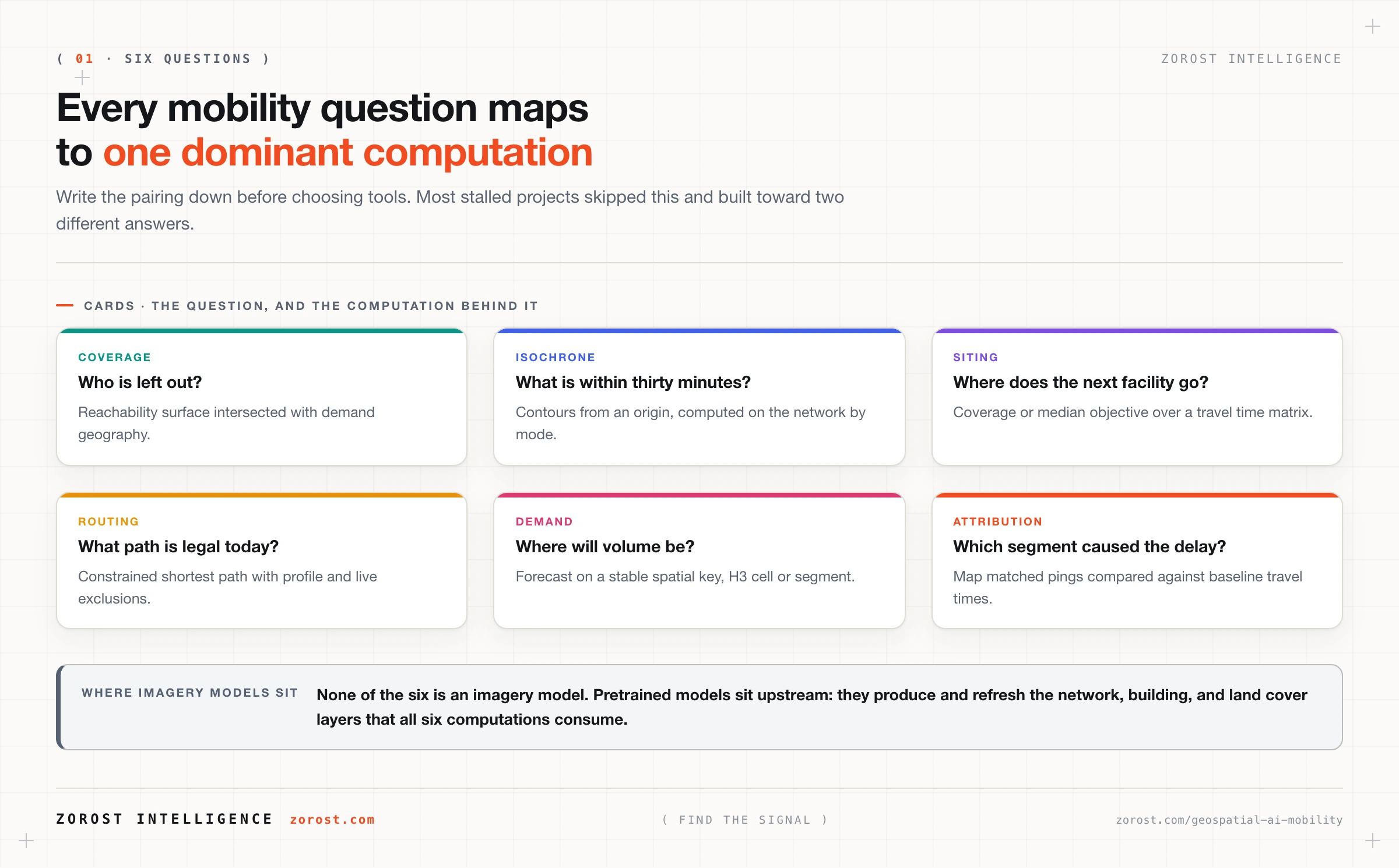
Six questions come up repeatedly, and each has one dominant computation behind it. Writing the pairing down early prevents the common failure of buying a tool that answers a question nobody asked.
| Operational question | The computation | What it needs |
|---|---|---|
| Who can we reach, and who is left out? | Reachability surface over the network, intersected with demand geography | Routable network, cost model, demand layer |
| What is within thirty minutes of this site? | Isochrone, one or more contours from an origin | Routable network, travel mode, time budget |
| Where should the next facility go? | Candidate scoring, a p-median or maximum coverage formulation over a travel time matrix | Origin to destination matrix, demand weights, candidate sites |
| What path is legal and feasible today? | Constrained shortest path with vehicle restrictions and live exclusions | Restriction attributes, closure geometry, vehicle profile |
| Where will volume be next month? | Forecast on a spatial unit, usually an H3 cell or a segment | Historical volume joined to a stable spatial key |
| Which part of the network caused the delay? | Attribution of observed travel time to segments through map matching | Position pings matched to segments, baseline times |
Two of these are network computations, two are optimisations on top of a network computation, one is a forecast indexed by geography, and one is attribution. None is an imagery model. That matters because imagery models get the attention, and they sit upstream of all six: they produce and refresh the layers the six questions consume.
Why does network analysis on a real route beat an abstract graph?
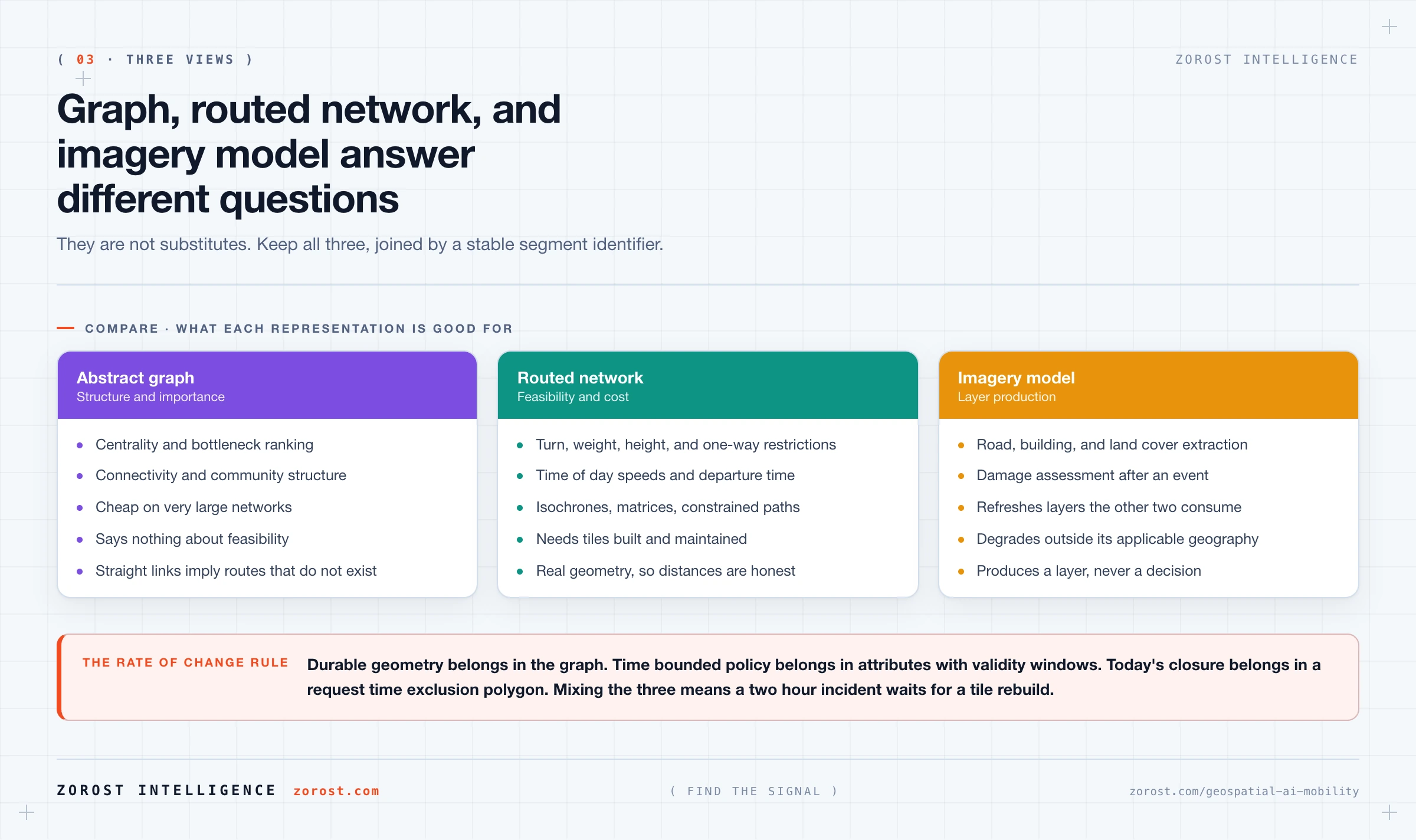
An abstract graph answers questions about structure and a routed network answers questions about feasibility, so you need both. Centrality, connectivity, community detection, and bottleneck ranking are properties of the topology. Whether a 44-tonne vehicle can make that movement at 07:00 on a Tuesday is a property of geometry and attributes that a topological abstraction throws away.
The gap shows up as soon as links stop being straight lines. A link between two ports follows a shipping lane, one between two rail yards follows track, one between two substations follows a transmission corridor. Drawing those as chords across a map produces a diagram that reads as connectivity but implies distances and pinch points that do not exist. Cambridge Intelligence added the fix to MapWeave in version 1.9.0 on 8 July 2026: a showRoutes option in the network layer that renders links along supplied route geometry, such as power lines, railroad tracks, or shipping lanes, while the data structure stays a graph you can analyse, recorded in their version 1 release notes. Graph and geometry are two views of one object, not a choice.
For the network itself, the open reference worth knowing is the Overture Maps transportation theme, which uses two feature types. A segment is a LineString for the centre-line of a path, carrying physical properties such as surface and width and non-physical ones such as access restrictions. A connector is a Point where segments meet, and topology comes from a connectors array on each segment, with the documentation explicit that each connector is a possible routing decision point. Their transportation guide also describes linear referencing, which lets a property apply to part of a segment without splitting the geometry in two.
Linear referencing decides whether your model can express reality. Speed limits that change by time of day, one-way streets that permit buses in the contraflow direction, and weight-restricted bridges with axle limits all apply to a portion of a path under a condition. A schema that splits geometry every time an attribute changes fragments the network until the identifiers become useless.
How do you compute an isochrone a planner will trust?
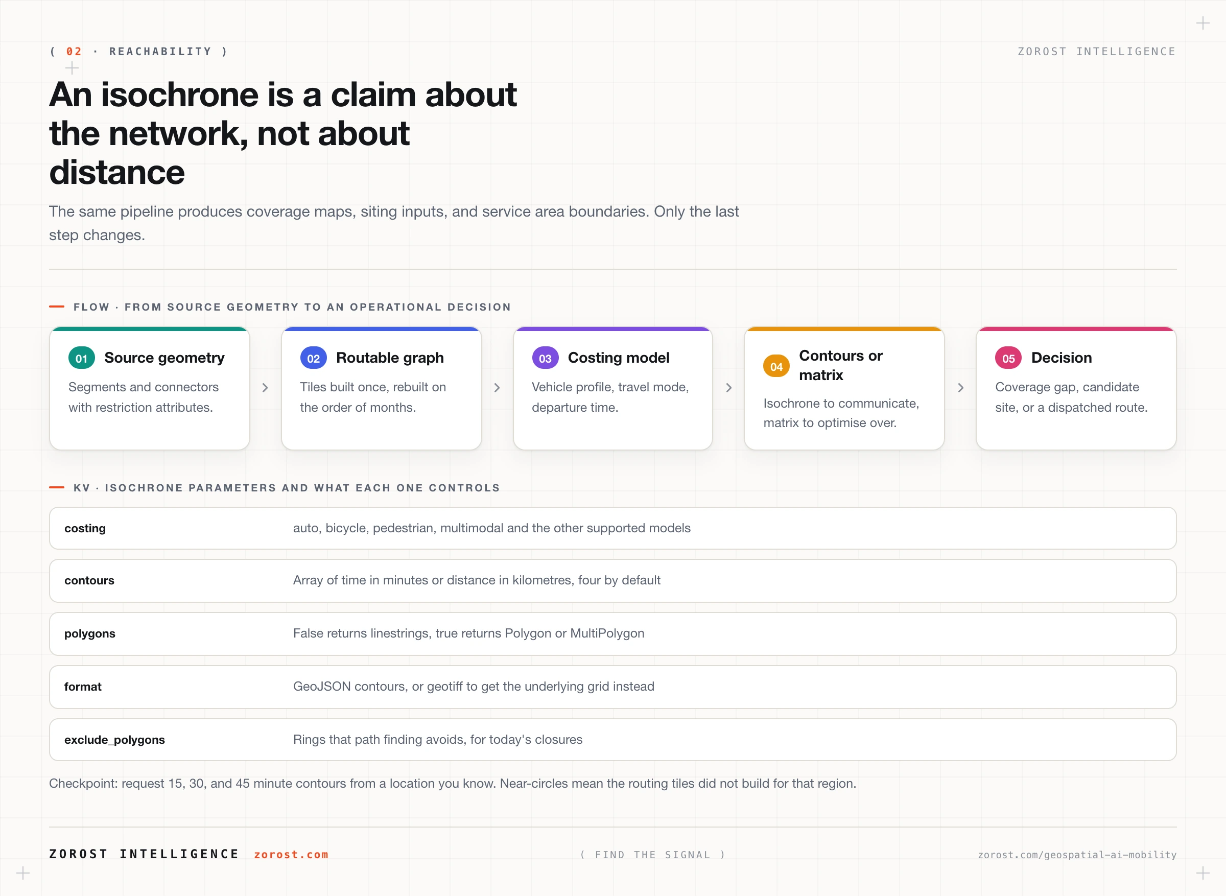
Compute it on the network with a costing model that matches the vehicle, and return contours rather than a radius. An isochrone is a line connecting points of equal travel time from an origin, and planners trust one over a buffer because the network is where the constraint lives: a river with two crossings, a rail corridor, an airport perimeter, a port gate that closes at 18:00.
Valhalla, the open source routing engine built on OpenStreetMap data, exposes this as an /isochrone endpoint, and its isochrone API reference documents the parameters that matter. You supply at least one location and a costing model, which can be auto, bicycle, pedestrian, multimodal, or another model the service supports, plus a contours array whose entries each give a time in minutes or a distance in kilometres, up to four by default. The polygons boolean decides output shape: the default false returns linestrings, true returns Polygon or MultiPolygon features. The response is GeoJSON derived from a two dimensional grid, and setting format to geotiff returns that grid instead, which is what you want when the isochrone feeds another raster computation.
Running locally, a request takes the form localhost:8002/isochrone?json={...}. The checkpoint that tells you the graph built correctly: request 15, 30, and 45 minute contours from a location you know well and confirm the shape follows the road network. Near-circles usually mean the routing tiles did not build for that region and the engine is working from a far sparser network than you expect.
For siting and coverage the companion endpoint is matrix, which computes travel time and distance between sets of locations. A siting question is usually an optimisation over that matrix rather than over isochrones: travel time from every demand point to every candidate site, then a coverage or median objective over the result. Isochrones communicate the answer; the matrix computes it.
Where do pretrained spatial models genuinely help?
Pretrained spatial models help when the task is a well-posed extraction from imagery and the training geography resembles yours. They produce or refresh a layer. Treating that output as a decision is the most common way this technology disappoints.
Esri publishes the largest catalogue. Its own guide in ArcNews states that ArcGIS Living Atlas of the World holds more than 100 pretrained GeoAI models, including Building Footprint Extraction for the USA, Road Extraction for North America, High Resolution Land Cover Classification for the USA, and a Damage Assessment model for drone imagery, each documented with its required inputs, training data, and expected performance. Read three fields on the item page before running anything: input imagery type and resolution, applicable geography, and expected performance.
Applicable geography separates a useful run from a wasted GPU day. A building footprint model trained on United States imagery encodes the roof shapes, materials, and parcel patterns of that built environment. Run it elsewhere and recall falls in ways that are hard to see at low zoom and obvious in the numbers. The documented answer is transfer learning: label a few hundred chips from your own imagery and fine-tune.
In transport work these models do layer maintenance. Road extraction refreshes a network where the authoritative source lags. Building and land cover extraction produce the demand and land use inputs a siting model consumes. Damage assessment after a storm says which parts of a network to treat as closed. The output is always an input to a network computation, so record which model version produced a layer, on which imagery date, at what confidence threshold. A route behaving oddly is often a changed layer rather than a routing bug.
How do you route under a constraint the map does not know about?
Separate the network into three tiers by how often each changes, and never encode a short-lived constraint into the graph. The durable network changes on the order of months, the restriction layer daily, the exclusion set hourly. A design that rebuilds routing tiles to reflect a two-hour closure will always be late.
The durable tier is geometry and permanent attributes. Overture’s transportation releases carry the relevant ones: maximum weight, height, width, and length access restrictions, one-way restrictions, and turn restrictions were added on the theme’s path to general availability. Those belong in the graph because they hold for months and a vehicle profile needs them at every routing decision.
The restriction tier is time-bounded policy: terminal curfews, seasonal weight limits, permit requirements, hazardous materials prohibitions on named corridors, and airport configurations that change with the operating day. Model these as attributes with validity windows, joined to segments by a stable identifier, and evaluate them at query time against the requested departure. A vehicle profile plus a departure timestamp then yields a different feasible network at 04:00 than at 16:00 without touching the tiles.
The exclusion tier is what happened this morning: a flood, an incident, a closed sector, a yard blocked by a derailment. Valhalla’s routing service takes an exclude_polygons parameter, one or more exterior rings supplied as nested coordinate arrays or a GeoJSON FeatureCollection, and roads intersecting those rings are avoided during path finding, as its route API reference documents. Temporary closures belong there: request scope, not graph scope.
The same split works in aviation, where the durable tier is runway, taxiway, and stand geometry, the restriction tier is published procedures and the day’s runway configuration, and the exclusion tier is whatever is closed right now. Zorost builds freight and aviation routing this way because with one graph encoding everything, every operational change becomes a data engineering change.
What does the data layer need to look like for any of this to work?
It needs three stable join keys, one storage format, and an evaluation set, and the absence of any one is usually why a pilot does not become a system.
The three keys are a network identifier, a spatial index, and a linear reference. The open option for the first is Overture’s Global Entity Reference System, which assigns stable identifiers to entities such as road segments and maintains them across releases with changelogs and bridge files back to source data, described in the GERS documentation. Match telematics or track data to a GERS identifier once and every later join is a column equality instead of a spatial predicate. The spatial index is H3 or an equivalent grid, for aggregation and coarse partitioning. The linear reference is an offset along a segment, which attributes an event to a point on a path without splitting geometry.
Storage should be GeoParquet, for the reasons in GeoParquet and the cloud-native geospatial stack: partial reads over object storage, bounding box statistics that let a bounded query skip most of the data, and one format a Spark job, a notebook, and a warehouse can all read. On Databricks, ST geospatial functions are available in Databricks SQL and Databricks Runtime 17.1 and above, with GEOMETRY generally available and GEOGRAPHY in Public Preview, and H3 functions have shipped since Runtime 11.2, so aggregation is plain SQL:
SELECT h3_longlatash3(lon, lat, 8) AS cell,
       date_trunc('HOUR', ping_ts)  AS hour,
       count(*)                     AS pings,
       avg(speed_kph)               AS avg_speed
FROM   vehicle_positions
WHERE  event_date BETWEEN DATE '2026-07-01' AND DATE '2026-07-07'
GROUP  BY cell, hour;
The evaluation set is the part that gets skipped. Hold out several hundred real completed trips with their observed durations, and score every change to the network, the costing model, or the layers against them, recording the graph build version and the model versions alongside each score. Without that you cannot distinguish “the routing got worse” from “the network was refreshed” from “someone changed the speed assumptions”, and all three happen in the same quarter. It is the discipline described in choosing by fit rather than fashion: name the measurement before the change, not after the argument.
Where this goes wrong
Buffers presented as reachability. The symptom is a coverage map that overstates service in exactly the places with a river, a rail corridor, or a restricted perimeter. The cause is a circular buffer standing in for an isochrone. Replace it with a network isochrone using the correct costing model, and expect the covered area to shrink noticeably.
Straight-line links on a map. The symptom is a network diagram implying routes and distances that do not exist, and a stakeholder inferring from a chord across water. The cause is treating the map as a canvas for a graph layout. Attach real route geometry to the links and keep the graph structure for the analysis.
Closures encoded into the routing graph. The symptom is operational changes queueing behind a tile rebuild, so routes are correct several hours after they mattered. The cause is one tier where there should be three. Move temporary closures to request-time exclusion polygons and time-bounded rules to attributes with validity windows.
Spatial joins where a key join belongs. The symptom is a nightly job whose runtime grows superlinearly as ping volume rises. The cause is repeating a point-in-polygon or nearest-segment operation that only needed to happen once. Map match to a stable segment identifier at ingest and join on the identifier thereafter.
No versioned evaluation set. The symptom is an argument about whether last week’s change helped, settled by whoever is most senior. The cause is that nothing was measured against held-out trips with versions recorded. Build the set before the first optimisation.
Common questions
What is the difference between an isochrone and a buffer?
A buffer is a fixed distance drawn around a point, ignoring the network. An isochrone is the area reachable within a travel time or distance budget along the actual network, computed with a costing model for a specific mode. Wherever crossings are limited, one-way systems dominate, or terrain constrains movement, the isochrone is substantially smaller and a different shape.
Do I need a graph database for network analysis on routes?
Usually not. A routing engine such as Valhalla builds its own tiled graph and answers path, matrix, and isochrone queries directly, and topology questions can be computed in a graph library over an extract. A graph database earns its place for traversing heterogeneous relationships that are not routing, such as shipment to carrier to customs event to facility.
What is map matching and why does it matter so much?
Map matching assigns a sequence of noisy position readings to the specific network segments a vehicle actually travelled. It matters because it converts continuous coordinates into a stable key, and that key turns every later question, such as segment-level delay attribution or lane-level volume, into an ordinary aggregation instead of a repeated geometric search.
Can a pretrained model replace an authoritative road network?
No, but it can keep one current. Road extraction models digitise geometry from imagery, which helps where the authoritative source lags reality, for example new industrial access roads or a reconfigured terminal. What they do not produce is the attribute layer routing depends on: turn restrictions, one-way rules, weight limits, access rules. Treat extracted geometry as a candidate change to reconcile.
Should I run my own routing engine or buy a routing API?
Decide on constraint expressiveness and volume, not price. A hosted API is the better choice when vehicle profiles are standard and query volume is moderate. Self-hosting an open engine wins when you need custom costing, unusual vehicle profiles, high matrix volume, or data residency over the routing requests themselves, which is common in government work.
Which spatial resolution should I aggregate to?
Pick the resolution at which the operational decision is made, then check the cell size against your positional accuracy. Aggregating finer than the accuracy of the underlying positions creates structure that is noise. For vehicle telematics and most facility-level decisions, an H3 resolution in the 7 to 9 range is the usual working area.
Next steps
Take one question your operation asks weekly, write down which of the six computations it maps to, and list the data each requires. Most stalled mobility projects are stalled because that mapping was never written and two teams are building toward different answers.
Then read the architecture decisions to settle before approving AI at scale, because a spatial platform commits you to a network source, a model layer, and an evaluation practice that are all expensive to reverse. For the storage layer underneath, GeoParquet and the cloud-native geospatial stack covers partitioning and the bounding box columns that make bounded queries cheap. The industries page shows where this work sits in aviation and freight.
The three-tier split between durable network, time-bounded restriction, and request-time exclusion is how Zorost builds routing and coverage work in freight and aviation, and we publish what we test in AI Fieldwork.